

Article Figures & Tables
Figures
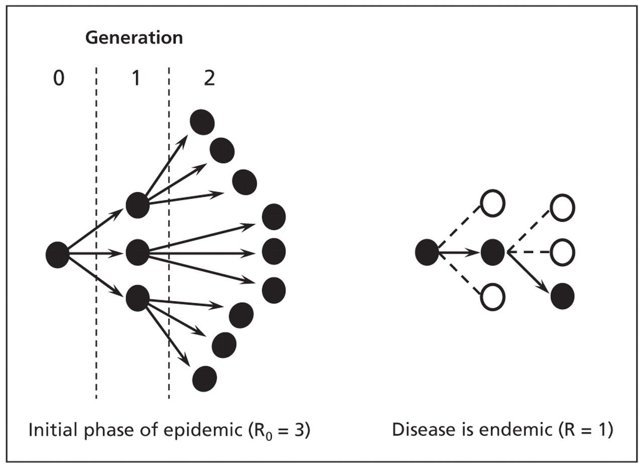
Figure 1: The number of new infections generated when the basic reproductive number (the number of new cases created by a single primary case in a susceptible population) is 3. Cases of disease are represented as dark circles, and immune individuals are represented as open circles. When there is no immunity in the population (left) and the basic reproductive number (R0) is 3, the initial infectious case generates on average 3 secondary cases, each of which in turn generates 3 additional cases of disease. Once the disease becomes endemic owing to acquired immunity (right), each case generates on average 1 additional case (effective reproductive number [R] = 1).
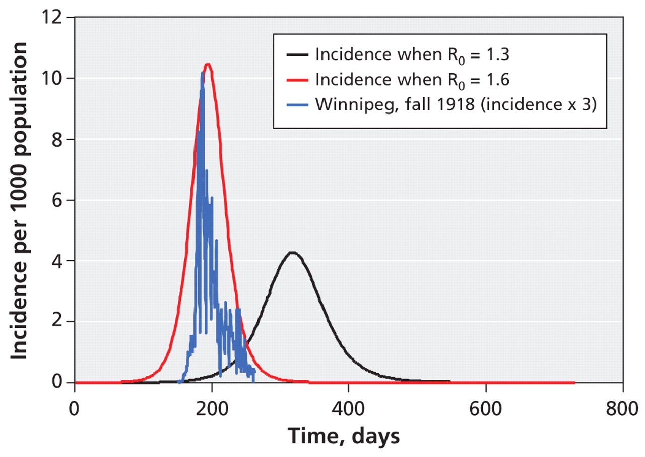
Figure 2: The effect of changing the basic reproductive number (R0) on the severity and duration of an influenza epidemic. A higher R0 (1.6, red curve) results in an epidemic with a higher peak incidence and a greater cumulative attack rate (not shown). When the R0 is lower (1.3, black curve), the epidemic peaks later, lasts longer and has a lower cumulative attack rate. The basic reproductive number of the disease is reduced through control interventions, including isolation of cases and “social distancing” (e.g., school closures). The blue curve represents actual incidence data from the autumn wave of the 1918 influenza pandemic in Winnipeg (multiplied by 3 for comparability of scales).
Figure 3: Possible effects of seasonality on a novel influenza strain. Panels show simulated epidemic curves when the basic reproductive number (R0) for influenza oscillates from 1.4 in winter to just under 1 in summer (black curves). When an epidemic emerges in winter (top panel), it is associated with a monophasic increase in prevalence (red curve). However, springtime emergence (bottom panel) results in a biphasic epidemic (red curve), as happened in the 1918 influenza pandemic. Cumulative attack rates are represented by blue curves. Prevalence data are multiplied by 10 for comparability of scales.


In this issue

Article tools


Jump to section
Related Articles
Cited By...
- Adapt or die: how the pandemic made the shift from EBM to EBM+ more urgent
- Model-based projections for COVID-19 outbreak size and student-days lost to closure in Ontario childcare centers and primary schools
- Mathematical modeling of COVID-19 transmission and mitigation strategies in the population of Ontario, Canada
- Modelisation mathematique de la transmission de la COVID-19 et strategies dattenuation des risques dans la population ontarienne au Canada
- Mathematical modelling of COVID-19 transmission and mitigation strategies in the population of Ontario, Canada
- The DAGs of war
- Transmissibility of the 2009 H1N1 pandemic in remote and isolated Canadian communities: a modelling study
- Modelling mitigation strategies for pandemic (H1N1) 2009
More in this TOC Section
Similar Articles
Collections